


New notebooks for Think Stats

Getting ready to teach Data Science in the spring, I am going back through Think Stats and updating the Jupyter notebooks. When I am done, each chapter will have a notebook that shows the examples from the book along with some small exercises, with more substantial exercises at the end.
If you are reading the book, you can get the notebooks by cloning this repository on GitHub, and running the notebooks on your computer.
Or you can read (but not run) the notebooks on GitHub:
Chapter 1 Notebook (Chapter 1 Solutions)
Chapter 2 Notebook (Chapter 2 Solutions)
Chapter 3 Notebook (Chapter 3 Solutions)
I'll post more soon, but in the meantime you can see some of the more interesting exercises, and solutions, below.
Exercise: Something like the class size paradox appears if you survey children and ask how many children are in their family. Families with many children are more likely to appear in your sample, and families with no children have no chance to be in the sample.
Use the NSFG respondent variable numkdhh to construct the actual distribution for the number of children under 18 in the respondents' households.
Now compute the biased distribution we would see if we surveyed the children and asked them how many children under 18 (including themselves) are in their household.
Plot the actual and biased distributions, and compute their means.
In [36]:
resp = nsfg.ReadFemResp()
In [37]:
# Solution

pmf = thinkstats2.Pmf(resp.numkdhh, label='numkdhh')
In [38]:
# Solution

thinkplot.Pmf(pmf)
thinkplot.Config(xlabel='Number of children', ylabel='PMF')

In [39]:
# Solution

biased = BiasPmf(pmf, label='biased')
In [40]:
# Solution

thinkplot.PrePlot(2)
thinkplot.Pmfs([pmf, biased])
thinkplot.Config(xlabel='Number of children', ylabel='PMF')

In [41]:
# Solution

pmf.Mean()
Out[41]:
1.0242051550438309In [42]:
# Solution

biased.Mean()
Out[42]:
2.4036791006642821Exercise: I started this book with the question, "Are first babies more likely to be late?" To address it, I computed the difference in means between groups of babies, but I ignored the possibility that there might be a difference between first babies and others for the same woman.
To address this version of the question, select respondents who have at least live births and compute pairwise differences. Does this formulation of the question yield a different result?
Hint: use nsfg.MakePregMap:
In [43]:
live, firsts, others = first.MakeFrames()
In [44]:
preg_map = nsfg.MakePregMap(live)
In [45]:
# Solution

hist = thinkstats2.Hist()

for caseid, indices in preg_map.items():
    if len(indices) >= 2:
        pair = preg.loc[indices[0:2]].prglngth
        diff = np.diff(pair)[0]
        hist[diff] += 1
In [46]:
# Solution

thinkplot.Hist(hist)

In [47]:
# Solution

pmf = thinkstats2.Pmf(hist)
pmf.Mean()
Out[47]:
-0.05636743215031337Exercise: In most foot races, everyone starts at the same time. If you are a fast runner, you usually pass a lot of people at the beginning of the race, but after a few miles everyone around you is going at the same speed. When I ran a long-distance (209 miles) relay race for the first time, I noticed an odd phenomenon: when I overtook another runner, I was usually much faster, and when another runner overtook me, he was usually much faster.
At first I thought that the distribution of speeds might be bimodal; that is, there were many slow runners and many fast runners, but few at my speed.
Then I realized that I was the victim of a bias similar to the effect of class size. The race was unusual in two ways: it used a staggered start, so teams started at different times; also, many teams included runners at different levels of ability.
As a result, runners were spread out along the course with little relationship between speed and location. When I joined the race, the runners near me were (pretty much) a random sample of the runners in the race.
So where does the bias come from? During my time on the course, the chance of overtaking a runner, or being overtaken, is proportional to the difference in our speeds. I am more likely to catch a slow runner, and more likely to be caught by a fast runner. But runners at the same speed are unlikely to see each other.
Write a function called ObservedPmf that takes a Pmf representing the actual distribution of runners’ speeds, and the speed of a running observer, and returns a new Pmf representing the distribution of runners’ speeds as seen by the observer.
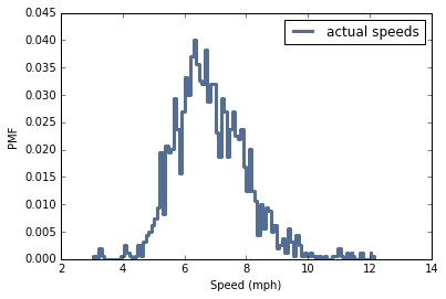
To test your function, you can use relay.py, which reads the results from the James Joyce Ramble 10K in Dedham MA and converts the pace of each runner to mph.
Compute the distribution of speeds you would observe if you ran a relay race at 7 mph with this group of runners.
In [48]:
import relay

results = relay.ReadResults()
speeds = relay.GetSpeeds(results)
speeds = relay.BinData(speeds, 3, 12, 100)
In [49]:
pmf = thinkstats2.Pmf(speeds, 'actual speeds')
thinkplot.Pmf(pmf)
thinkplot.Config(xlabel='Speed (mph)', ylabel='PMF')
In [50]:
# Solution

def ObservedPmf(pmf, speed, label=None):
    """Returns a new Pmf representing speeds observed at a given speed.

    The chance of observing a runner is proportional to the difference
    in speed.

    Args:
        pmf: distribution of actual speeds
        speed: speed of the observing runner
        label: string label for the new dist

    Returns:
        Pmf object
    """
    new = pmf.Copy(label=label)
    for val in new.Values():
        diff = abs(val - speed)
        new[val] *= diff
    new.Normalize()
    return new
In [51]:
# Solution

biased = ObservedPmf(pmf, 7, label='observed speeds')
thinkplot.Pmf(biased)
thinkplot.Config(xlabel='Speed (mph)', ylabel='PMF')

In [ ]: